Modifying Cell Format

Description

Applying formatting and styles of cells in our Excel workbooks is important to maintain a clean and clear format. In this article, you will learn how to format cells in an Excel file.

Instructions

Here’s how to do it in a few easy steps:

1. Create the VBS script with the instructions needed
2. Save the VBS file in the root folder of the project
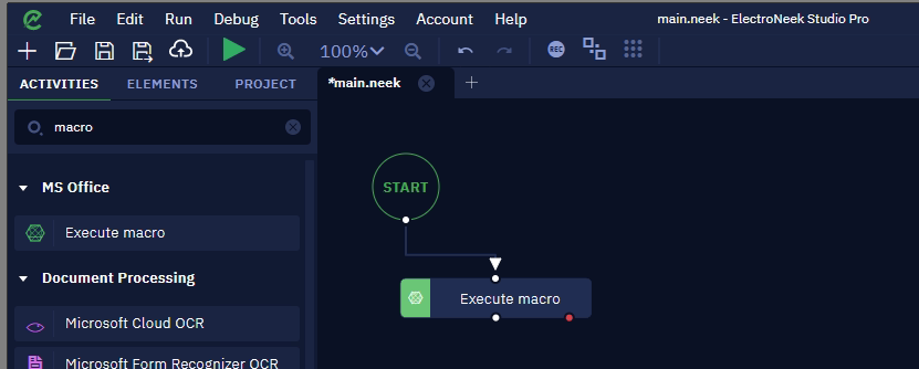
3. Use Execute Macro activity and set the parameters

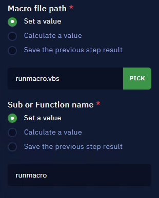
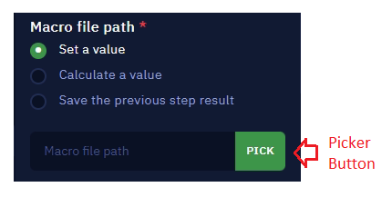
3.2. Set the VBS script path using the picker button or using the Calculate a value option following the JS methods for handling strings

🚧

Caution

Be careful with JavaScript escape characters when working with strings.

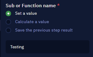
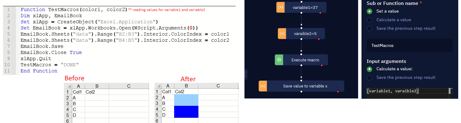
3.3. Enter the name of the function without the parentheses. For example, if a Sub Testing() function is created, just enter Testing

3.4 Run the workflow.
The expected result is saved within the Excel file. To validate it, it is necessary to open the file.

For example, to change the background color of a cell or group of cells, use the "ColorIndex" property. To do so, declare the color-index in a variable and then pass it using the "Input arguments" field of the Execute Macro activity.

📘

Tip

In cases where the script returns a value, you need to use the Assign value to variable activity to save the result.

When creating the VBS script, try to use the Late Binding methodology.

⬅️

Back to the table

---

Reading rows in a loop

Description

To process an Excel file, it is common that we need to read the row values from a particular column one by one on a loop. For example, imagine you have a column consisting of keywords that you want to input in the browser and extract the search results for those keywords one by one.

Good news: we have a specific activity to perform that task — it is called For each row.

Still, it may be possible that, for some reason, you are required to execute the steps manually in another workflow. So, here is a quick step-by-step content to guide you throughout this process.

Instructions

First of all, follow these steps:

1. Read the contents of the Excel file using the Read Excel file activity. The values of the Excel file will be stored in the variable "excel_content"

2. Create a variable called "counter" using the Assign value to variable activity and assign the "0" value to it

3. Then, use the If…then activity. Bear in mind that:

• The activities you place below it need to be executed on a loop to read the row data from the variable "excel_content" one by one
• The conditions provided should be counter < excel_content["Sheet1"].length
• The excel_content["Sheet1"].length returns the highest count of the row from the Excel file
• The values in the variable "excel_content" are stored as an array, hence you have to start the loop from "counter = 0"

4. Next, add the Console log activity to print the row values one by one

5. Select the "Calculate a value" parameter for the Message option. The syntax to read row-wise data from the Excel file is excel_content[Sheet Name][Row Number][Column Name]. Hence, we must use excel_content[Sheet1][counter]["A"] (keeping in mind that the value of the variable "counter" here is 0)

📘

Tip

In the Read Excel file activity, if you have used "Use table headers" as the "Get dictionary key" value instead of "Use column letters", the syntax must be excel_content[Sheet Name][Row Number][Table Header Name]

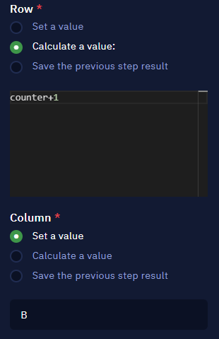
6. To loop through each row value, it is essential that we iterate the value of the variable "counter" — that is, we must repeatedly input that value. So, in the Assign value to variable activity that comes after the Console log activity, select the "Variable value" as "Calculate a value" and enter the value counter + 1

7. Once done, connect the Assign value to variable activity to the If…then activity so they form a loop

8. Now, run the workflow — you will see the row values getting printed in the console one by one.

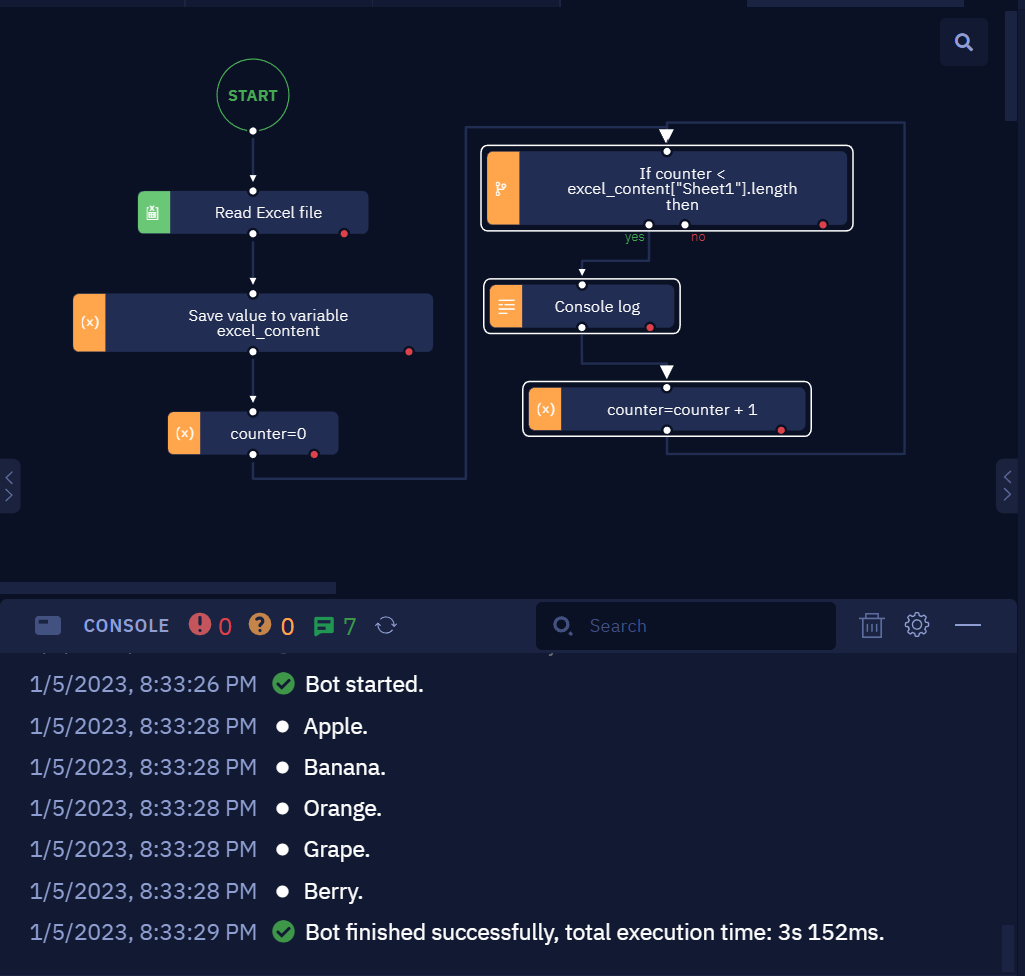
As you can see, the logic of the workflow is quite simple.

📘

Note

Still, keep in mind that using the For each row activity you can perform the whole process in just a few clicks.

⬅️

Back to the table

---

Removing Blank Rows

Description

Keeping an Excel file clean improves the execution time of our bots. Also, some activities may fail or take longer than needed if entire rows are blank.

In this article, you will learn how to delete empty rows or lines from Excel worksheets using the Remove empty rows activity. The benefit of this action is that, for example, when the For each row activity is executed in a workflow, it does not take time to process blank rows unnecessarily.

Instructions

Here’s how to manage empty rows in a few easy steps:

1. Read the Excel file with any of the following activities: Read Table, Read Excel File, Read Excel Range.

2. Use the Remove empty rows activity to remove empty rows.

3. Save the results of the previous step in a variable.

4. You can then save this variable back to a new Excel file or perform other activities on this data, like For each row.

📘

Note

There are 2 conditions for removing empty rows:

• Each cell in a row is empty — it removes all rows with all empty cells.
• At least one cell in a row is empty — it removes all rows with at least one empty cell.

🚧

Caution

Incorrect handling of empty lines in excel files can generate the exception "EBUSY: resource busy or locked, unlink".

⬅️

Back to the table

---

Merging Table Data

Description

In this article, you will learn how to create a workflow using one method to merge 2 Excel spreadsheets with the same columns into 1 file. Find the downloadable files we used at the end of this document.

Instructions

Here’s how to do it in a few steps according to the activities you choose. We offer you two different combinations in the following instructions.

Merging spreadsheets content with Read Excel File and For Each Row Activities

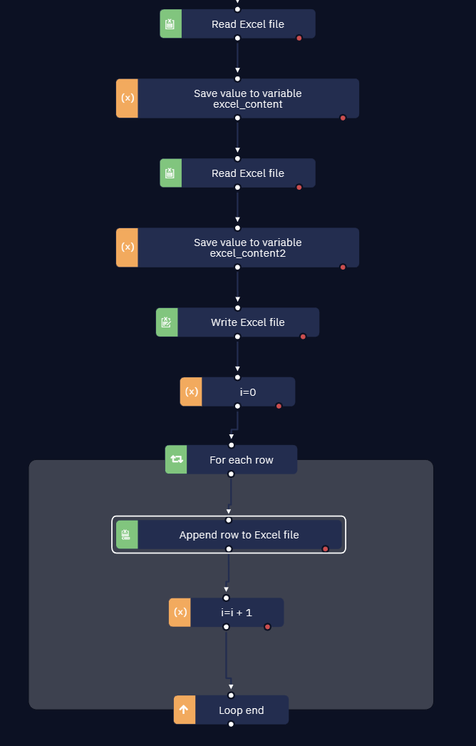
1. Read the first Excel table using Read Excel File.

2. Read the second Excel file also using Read Excel File activity and save the results in different variables.

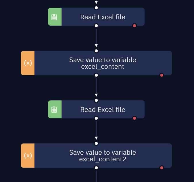
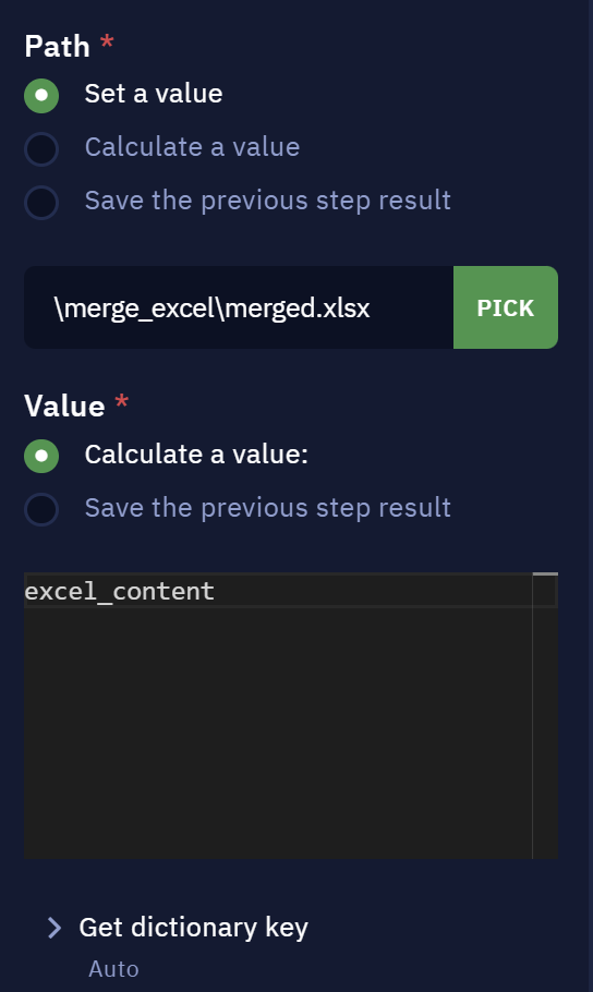
3. Create a third Excel file that will be the result of the merge, inside this Excel file add the content of the first Excel file that was read.

4. Now use the For each row activity but first, it's necessary to create an Index, and inside of the “For each row“ add +1 in the index.
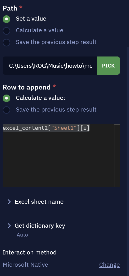
5. Also, inside the For each row activity insert the Append row to Excel file activity with the following value: excel_content2["Sheet1"][i].

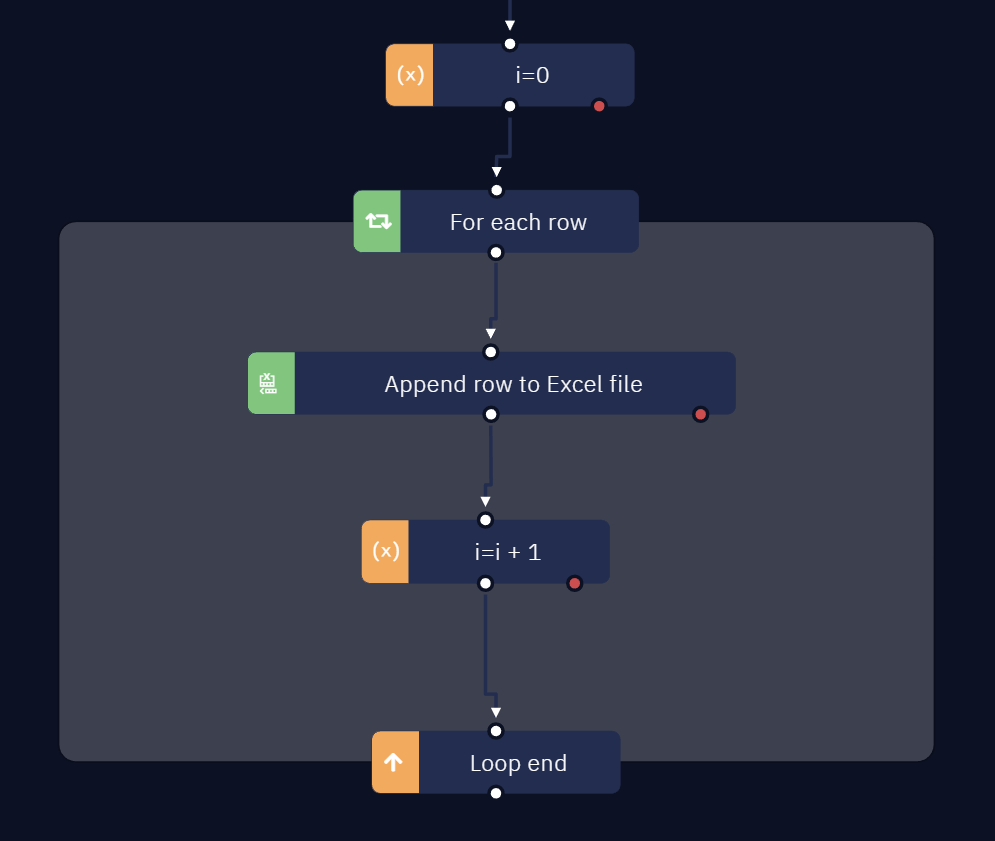
6. Finally, the complete workflow should look like this screenshot.

Merging spreadsheets content with Read Excel Range and Write Excel Range Activities

First, read the table from the second file using Read Excel Range.

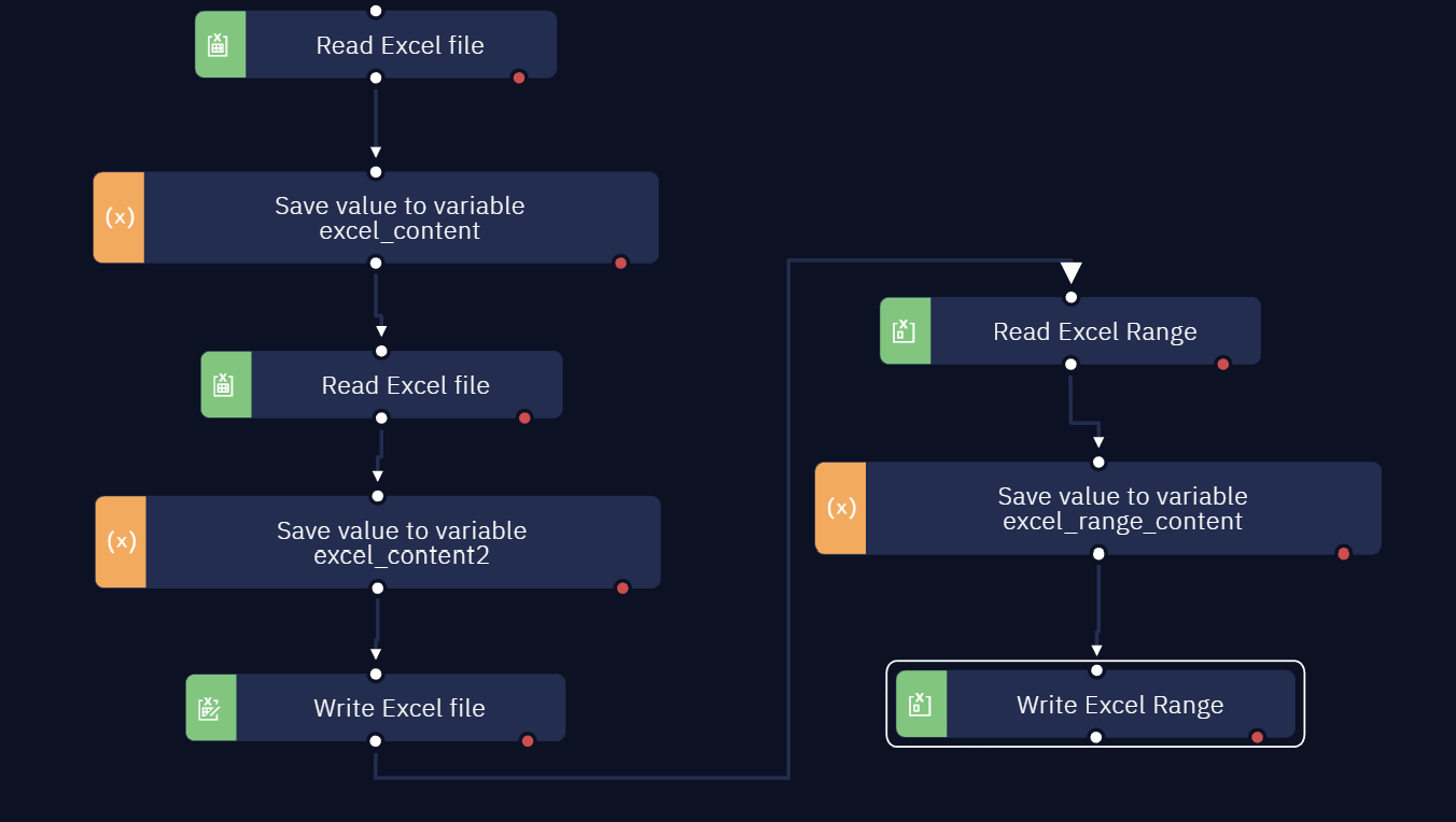
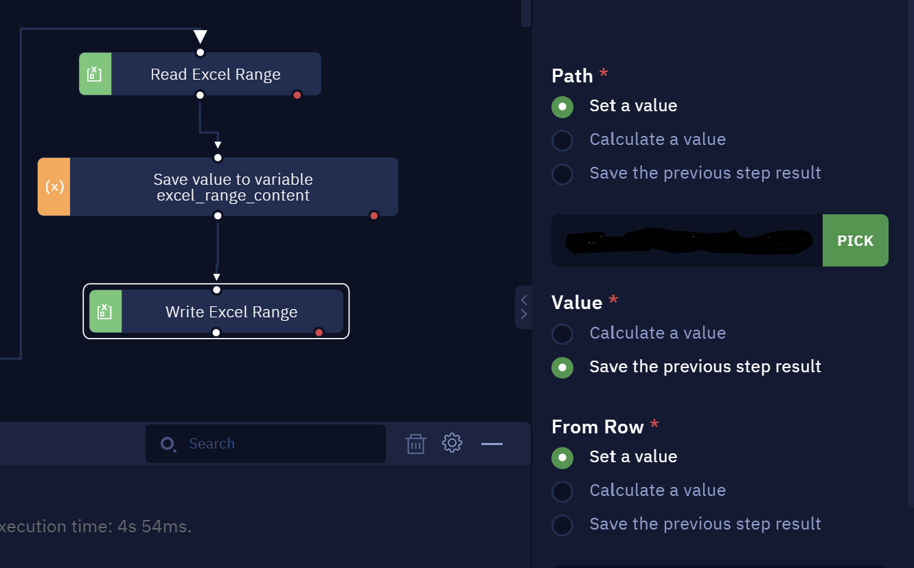
2. Then, select the Write Excel Range activity to insert the value in the created file.

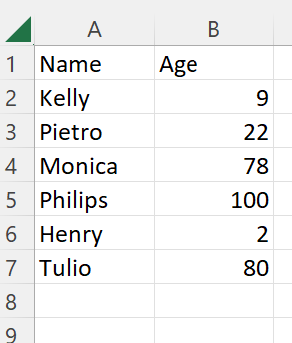
3. The resulting table will look like the following screenshot.

🚧

Note

The Excel Generic Library may have faster results.

⬅️

Back to the table

---

Using conditional formatting with Macros

Description

There are cases when you want to implement conditional formatting in an Excel file. For example, you would like to highlight all the values that are less than "0" in red for a particular column.

In this article, you will learn how to apply conditional formatting while using the Execute macro activity in Studio Pro.

Instructions

Here’s how to do it in a few steps:

1. Follow the instructions provided in the Execute Macro article.
2. Copy and paste the VBScript below that shows how to highlight all the values less than 0 in red for the range A1:A40.

Sub TestMacros()  
Dim rng, fc, xlApp, EmailBook  
Set xlApp = CreateObject("Excel.Application")  
Set Book = xlApp.Workbooks.Open(WScript.Arguments(0))  
Set Sheet = Book.Sheets("data")  
Set rng = Sheet.Range("A1:A40")  
Set fc = rng.FormatConditions.Add(1, 6, 0)  
fc.SetFirstPriority  
With fc.Interior  
.Color = RGB(255, 0, 0)  
End With  
fc.StopIfTrue = False  
Book.Save  
Book.Close True  
xlApp.Quit  
End Sub

🚧

Note

The above VBScript can be modified to include another conditional formatting as well.

⬅️

Back to the table

---

Managing Large Files

Description

When dealing with big-size files, we may need to split them in order to read all their content.

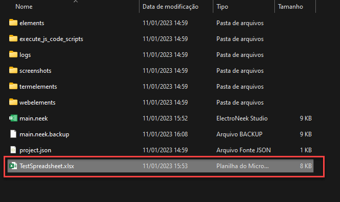
In this article, you will learn how to split large Excel files. We are going to use the file at the end of this document as an example.

Instructions

Here’s how to do it in a few steps:

1. Create a new Project in Studio Pro.
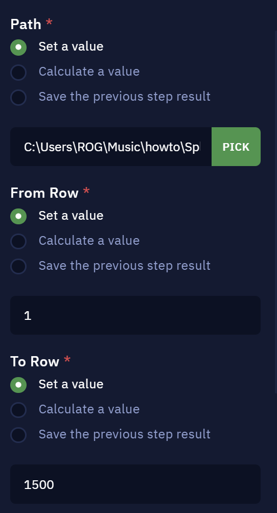
2. Insert the Read Excel Range activity.

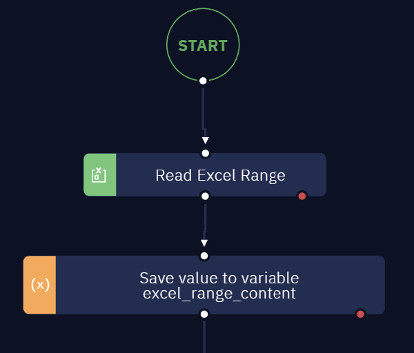
3. You can split the file as many times as you need. In this particular example, we are going to split it into 2. As the file contains 3,000 rows, we suggest first reading 1,500 lines and then the next 1,500 lines. So, enter the "From row" value as 1 and the "To row value" as 1500.

4. Repeat this procedure one more time.

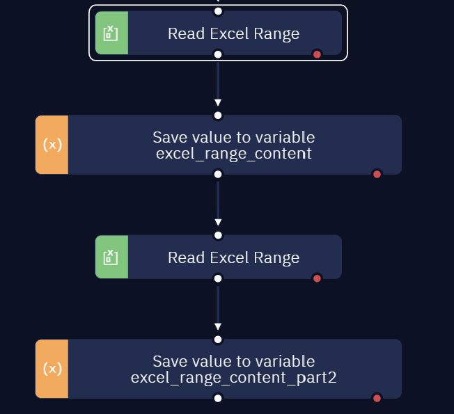
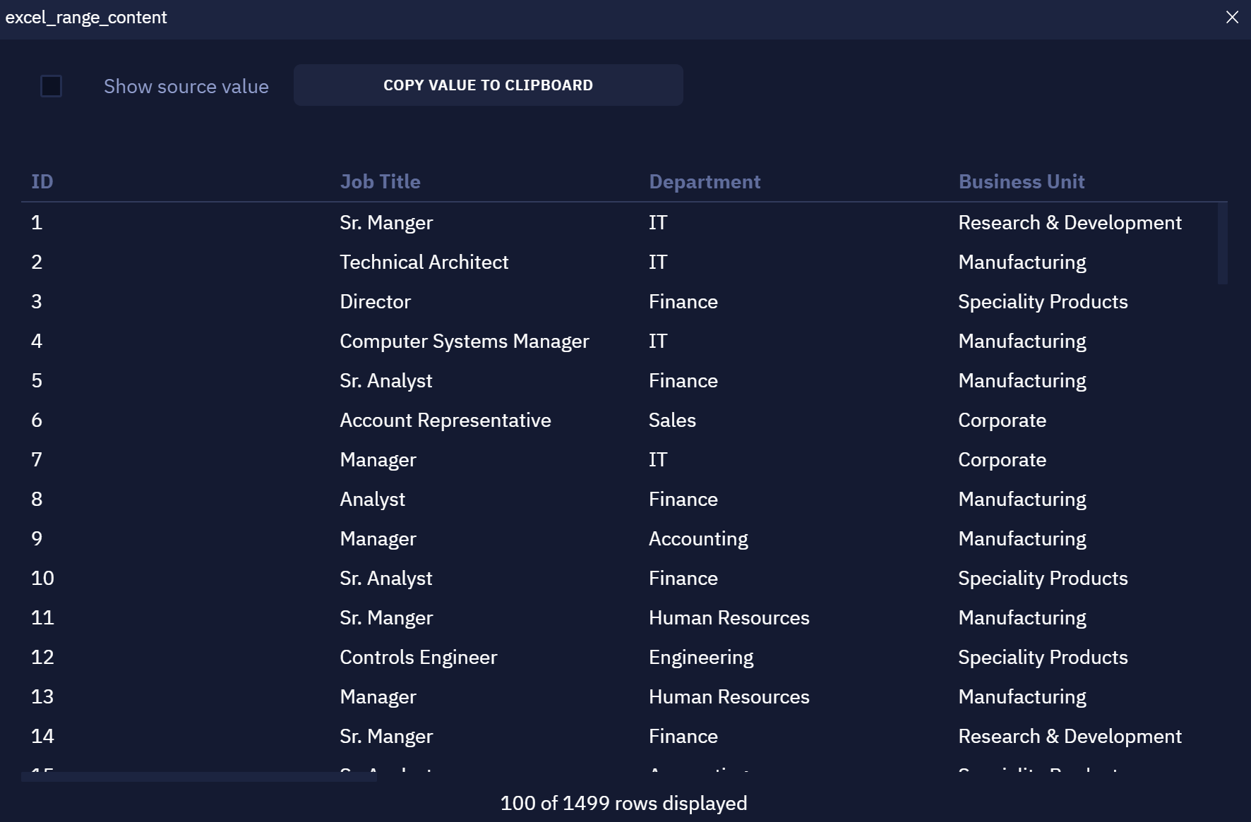
5. As a result, you obtain two separate variables with the values you previously set. Look at the screenshots below.

⬅️

Back to the table

---

How to add Excel functions to cells in a spreadsheet

In this article, we'll guide you through the process of integrating Excel functions into specific cells within a workbook. Our example will focus on using the VLOOKUP function between two sheets.

Setting up your environment

To begin, ensure that the Excel workbook containing both data and functions is stored in a location accessible to your automation process. For this guide, let's assume the workbook is situated in the project's root folder.

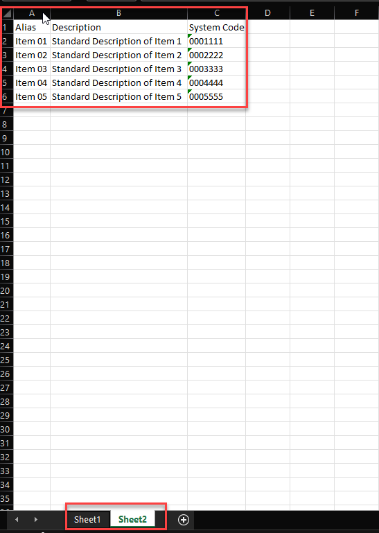
Our example centers on the practical use of the VLOOKUP function, a fundamental tool for Excel users. Consider a workbook with two sheets:

• Sheet 1: This sheet is where you'll integrate the Excel functions.

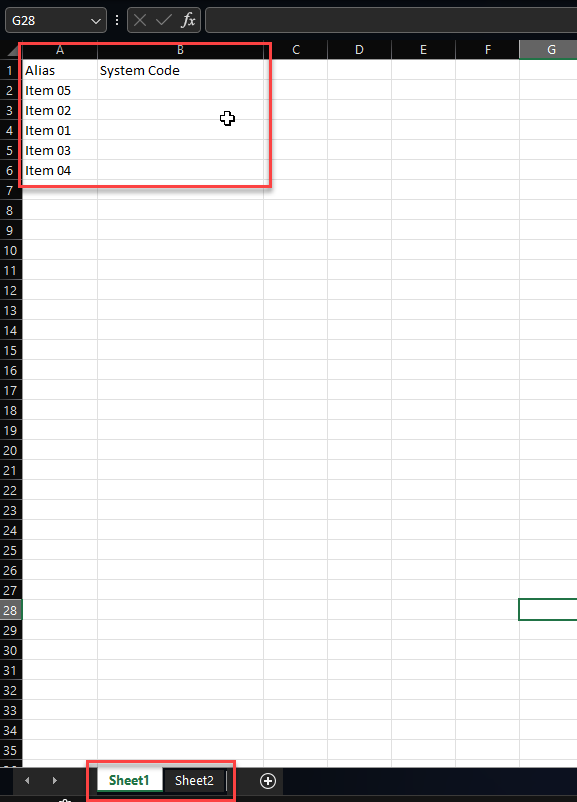
• Sheet 2: It holds the data referenced by the functions.

Scenario 1: Updating a Single Cell

Follow these steps to update a single cell using an Excel function:

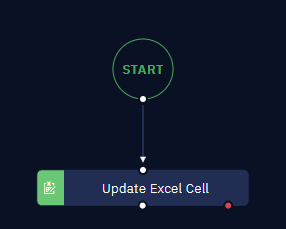
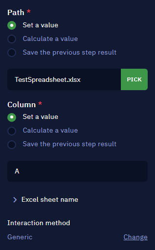
1. Open ElectroNeek Studio Pro and add the "Update Excel Cell" activity.

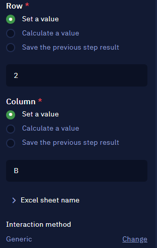
2. In the Properties Tab, provide the required information:
   • Path: The path to the workbook file.
   • Value: The function you want to use.

• Row: Specify the row number for the update.
• Column: Indicate the column to update.
• Interaction Method: Choose between Generic or Native interaction methods based on your needs.

📘

Note

Learn more about Updating an Excell cell in this article.

Scenario 2: Dynamic Column Updates with Excel Functions

For situations requiring dynamic updates across an entire column, follow this approach:

1. Start by reading the Excel workbook containing your functions.
2. Extract the number of rows within the worksheet.

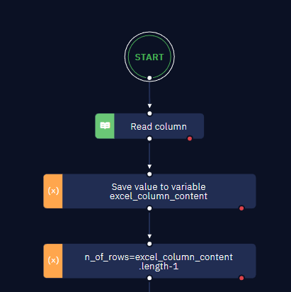
3. Create a loop that iterates through each row, updating the relevant cell.

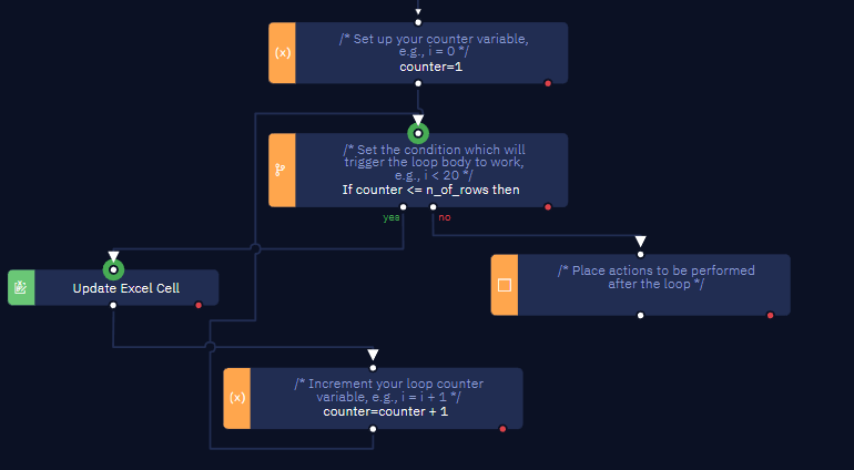
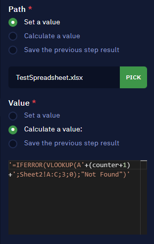
4. Set the Path to the workbook.
5. In the Value property, utilize the "Calculate a value" feature. Insert the function syntax, incorporating a counter variable to adjust the function's position for each row.
6. Similarly, use the "Calculate a value" option for the Row property. This ensures the row number for the update is incremented.

📘

Note

Keep in mind that the Excel function syntax must be in English.

⬅️

Back to the table

---

How to run VBA scripts through Studio Pro

In certain situations, you might need to execute macros with native Excel functions, and this is not supported by Visual Basic Script (.vbs).

Instructions

1. Open a New Excel Workbook.
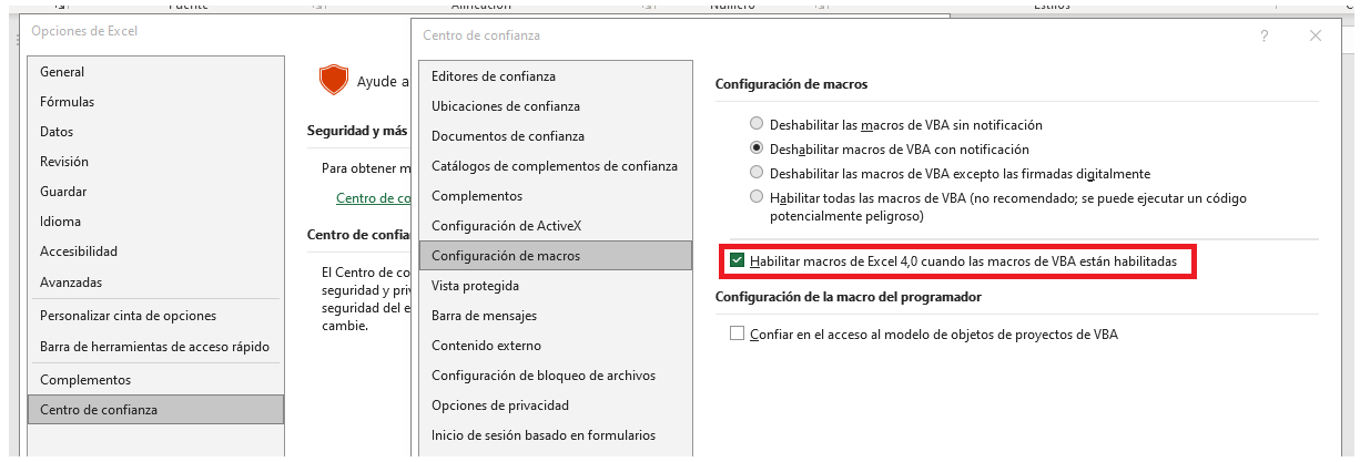
2. Go to File > Options > Trust Center.
3. Click on "Trust Center Settings..."
4. Under "Macro Settings," make sure to check "Trust access to the VBA project object model."

5. Create your Excel Macro VBA Script.
6. Copy the code and use a text editor to save it with a .bas extension.
7. Create a VBS File with a function that calls the previously saved .bas file.
8. Configure VBS Script in Studio Pro.

⬅️

Back to the table

---